Visualization of the solution
Near-field and far-field
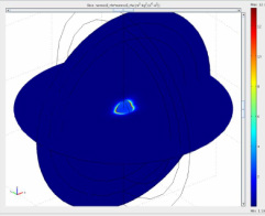
Fig.1 Intensity of the scattered field by gold nanoparticle in resonance. Notice enhancement factor and localization typical for dipolar resonance. (CLICK to ENLARGE)
Figure 1 shows plot of intensity of scattered field by our metallic
nanoparticle in resonance condition. Resonance condition can be assumed
to be around 510nm, but it can be extracted after far-field calculations
(See below.)
What we can say about this solution? At first sight, since we recognize dipolar pattern corresponding to x polarized plane wave excitation, we might think that is ok. However, few more thing can be checked, such as PML performance, meshing finesse and excitation definition.
Since we are sure that PML´s ref.ind. is same as nanoparticle surroundings, we should not get any parasitic reflections in ideal case.
How to chose PML´s thickness? This is not so clear, but my experience (although might be not entirely true) points to the thickness that is required for efficient scattering wave damping. When using swept mesh, 5 elements is just fine, and as a rule of thumb, if your mesh element on the other side of inner PML boundary is 10nm, then you should keep the same length of PML meshing elements, thus we can go to 50nm. Usually this works. IF YOU USE verion OLDER than 3.5a plus some hotfix update, you might expect that default PML will just not work. You will encounter reflections of the order of 10% of the excitation.
To test if your PML works, simply remove metallic nanoparticle by turning it into air (n=1), and solve the system.Plot one of the components of the scattered field (scEx_rfw, scEy_rfw or scEz_rfw). Check what are the max/min values, if your excitation is 1V/m, then expected amplitude for scE components should be less than 0.1% of excitation amplitude, depending on mesh and PMLs. If you refine mesh more you should get 10pow(-5), if your analytically described excitation is the solution of the empty model (in uniform air environment the definition is trivial) (Fig.2.b)). If you are getting some reflections of the order of 1-10%, most likely default PML doesn´t work, so you need to update it to COMSOL 3.5a, and then to patch it. Other option is to set your PML as regular domain, and then to define its parameters as your own PML, but I will not deal with that here.Playing with other parameters ("absorbing in r direction") will not get you anywhere.
Now we will take a look at far-field variable calculated by implemented Straton-Chu formula. Figure 3.a) shows plot of far-field on the spherical boundary. It exhibits dipole emission pattern driven by x-polarized incident field. To calculate scattering cross section, one should integrate square of far-field variable over some enclosed spherical surface. The fastest is to choose the surface of the colloidal nanoparticles. Why? Straton-Chu calculates the far-field variable defined on some boundary. If you take a look on math. expression of Straton-Chu (see section Straton-Chu), it is integral of the field over some surface enclosing the scatterer, that expresses the field in the infinity in the direction of the normal of the surface. Thus, since here the integral is solved for every mesh element on that boundary where far-field variable is defined, smaller the surface, less mesh element we have, and it is faster to calculate it. Note that the value of the integral has to be normalized by surface of the sphere used for the definition. For more info, follow the next link:
http://iopscience.iop.org/1367-2630/10/10/105006
Here you can find the correct expression for scattering cross section. If you are interested only in the resonance location, integrating square of the far-field variable is just fine. Also, there is an expression for absorption cross-section, which is proportional to the integral of the resistive heating over the nanoparticle volume. Generally, these two give extinction cross-section, and these two peaks might not entirely overlap[]. Resonant condition depends linearly on refractive index around particle, with red-shifting of resonance with higher refractive index, as shown in Fig.3.b) and c). For vacuum case, resonance is at 520nm, while in water is at 565nm. Note that resonance peak of scattered field is imposed on Reyliegh scattering curve that scales as 1/pow(Lambda,4), and that figures b) and c) are showing different wavelength range.
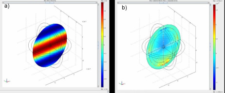
Fig.2. shows plots of two variables. a) Analytically defined excitation exp(-j*k0_rfw*nair*z) COMSOL does not solve b) x-component of scattered field without scatterer. Note the max/min values, and compare to max/min values of the a)
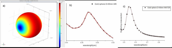
Fig.3. a) Dipole emitting pattern for x-polarized resonant excitation(far field variable) b) Scattering cross-section for gold colloid (60nm diameter) in air. c) Far-field spectra of the same nanoparticle in water exhibits red-shifted resonance. (Note: Resonance dependence of nanoparticle to the surroundings can be utilized for bulk refractive index or bio-molecular sensing)
