Visualization of solution
Testing excitation definition
1. Plotting excitation
After solving we can visualize analytically defined excitation (it is not dependent variable, thus not solved by solver). By plotting excitation we can only check if there are serious errors in our excitation. First, we can check if wave fronts correspond to plane wave. Also, after Snell´s law, we know that if wave is incident from the optically denser medium (higer refractive index), the refracted wave will emerge under bigger angle. This is demonstrated in Fig.1, where a) is excitation in case of coarse meshing, and b) when meshing is considerably finer.Only smoothness of the wave fronts can indicate not sufficient meshing, but you should not in general rely on this parameter.
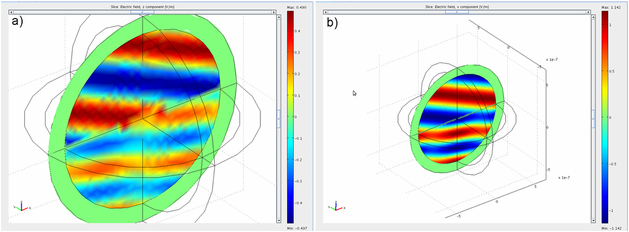
Figure 1. Plot of analytical definition of the incident fields.This variable is not solved by COMSOL. Every mesh element takes value according to the definition, so coarse meshing can give grainy plot. This however should not be used as indication of mesh quality.
2. Plotting scattered field
The more important parameter that can indicate if everything in the model is fine, is plot of scattered fields components. Since there are no scattering objects and analytical defined excitation is the solution of the geometry by definition, scattered field should be very small, in the range of numerical error. The good indication of the lack of meshing quality is amplitude of the scattered components. Our excitation fields are defined to have amplitude of sqrt(2)=1.41 V/m, 1V/m each component for p-polarization (check Fresnel´s coefficients page). Figure 2. a) shows x component of the scattered field, and maximum (minimum) amplitude is 0.0127V/m, i.e. around 1.2%. When we refine mesh to some extent, amplitude falls to 0.000124V/m. This is much better situation. Generally, this is usually indication of good meshing. If I remember well, in the manuals and comsol documentation, scattered field amplitude of 0.00001 is just enough, and it corresponds to numerical error.
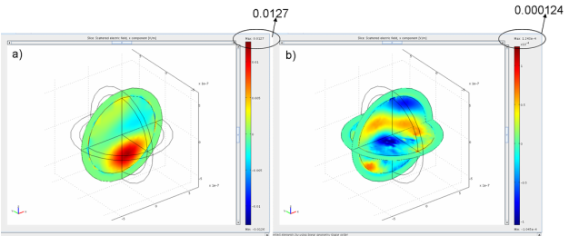
Figure 2. Scattered field components after solving scatterer-free interface problem. Not that amplitude of the scattered field depends on the meshing quality (among other parameters), and that ideally should be zero. a) coarse mesh b) finer mesh
3. Problem of wrong excitation definition
If you make a mistake in defining excitation, or in typing the analytical expression, depending on the difference between the actual solution of your geometry and the definition, calculated scattered field will be smaller or larger. For instance, if we omit transmitted wave in the definition (Fig.3 a)), the corresponding x-scattered field amplitude maximum goes to 1.298 V/m, which is higher than the amplitude of the incident field. Thus, if your definition is more similar to correct solution of geometry without scatterers, scattered field will go to very small values. For instance, if you work with normal incidence on glass/air interface, omitting Fresnel coefficients will not be that serious problem (reflection is only 4%). If you do the same for glass/water interface, error will be smaller, maybe even negligible. If you want to simulate multilayer films, than scattering formalism is only for the toughest, i.e. theoreticians.
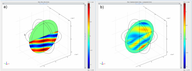
Figure 3. a) Plot of badly defined excitation. In the definition of the incident field, refracted wave was omitted by purpose to demonstrate its affects. b) Correspondent scattered field after solving a). Note that parasitic reflections are even stronger than the incident field.
4. Badly defined PML
In COMSOL versions earlier than 3.5a without hotfix patch, default PML definitions are wrong. What was the problem I don´t remember, but if you choose proper thickness of your PML, right refractive index and nice meshing, still amplitude of scattered field might be high. Trying to optimize thickness of the PML and "absorbing in r-direction" parameters will not take you anywhere. One of the solutions is to define your own PMLs, but that is not in the scope of this tutorial. Other solution is to forget about scattering-field formalism, and to try to solve your problem when total field is dependent variable (I am not sure if PML is working fine when solving total field in earlier versions-never checked this). Also you can ask comsol support to provide you with the patch, even if your license has expired long time ago, cause that is the serious software bug. Third solution is to change your geometry in a way that these parasitic reflections are located somewhere in your geometry where they are not affecting your solution, but this should be the last option.
5. Conclusion
Now it is clear how you should make you model. After drawing geometry, and defining all sub-domains and boundaries, you should turn your scattering objects into medium that surrounds them, and check if previously meshing is dense enough, or if your PML is working fine or if your definition of the exciting field is correct. After solving the geometry, check amplitudes of the scattered field, and if they are small enough, make your scatterers active, and solve the problem. Later, you might tune meshing of the scatterer, position of the integrating surfaces for far-fields, or size of your domain. That will be partially covered by Example 3.
