PORT Boundary Condition
Port BCs are very important and useful when working with total field. User guide doesn´t provide us with very useful information (what a surprise!) and above all, many of users just avoid reading them, and try out iteratively to set parameters until they figure it out. The best is to make some compromise, read manual and use trial-error procedure.
Port BC are used as boundaries for launching excitation into geometry when solving for total field. Why are they better than SC BC with excitation?
1) You can use them to launch different guided modes, by only setting very few parameters, like mode number in case of slab-waveguide, or fiber.I have never tried this, but if it works as I have just described, it is not bad. Although, I would first solve propagation constants in separate model, just to be sure.
2) As most important way of defining excitation will be user defined (not by mode numbers), the way of doing it is very similar to SC BC. However, there is one huge advantage over SC BC. When working with assemblies and identity pairs, you cannot use SC BC inside your geometry to define excitation at interior boundary, within geometry enclosed by PMLs.
Since defining excitation by PORT BCs can be somewhat ambiguous, I will start form the beginning whit simple 2D model..
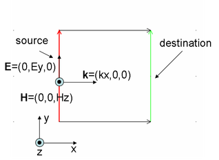
Fig. 1. 2D geometry used to demonstrate PORT BC setting up. TM plane wave travels form left (source) to the right (destination).
In-plane TM waves model was selected, and square is used as modeling space. Aim is to simulate simple free space propagation of plane wave in vacuum. K vector is parallel to x-axis. Top and bottom boundaries should be chosen in order not to spoil the wave propagation. Since we know that there is only electric field component normal to the top and bottom boundary, condition nxE=0 is satisfied, so we choose Perfect Electric Conductor BC (PEC). What remains is to set excitation.
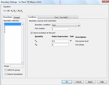
Fig.2. First window that opens up when setting PORT BC. We can set port number, as well as INCIDENT POWER and phase.
Fig.2. shows window for setting BCs. Each port needs unique port number. Incident POWER can be set. Port phase is disregarded, when using USER DEFINED mode specification, because phase is determined by your mathematical expression. If you click Port tab, there you can set remaining parameters. If you set H0z to be 0, then there will be no field at all. Any other number you set, it will be disregarded. Propagation constant is component of k vector that is normal to the boundary. If there are other components, they go in H0z field, where only constant part is disregarded, exponential part is taken into account (at least I hope, otherwise these all edit fields make no sense).The amplitude of our Hz component as well as Ey component is determined from input power according to E x conj(H) * d=E0*E0/2η0*d*cos(theta) (line integral of Poyinting vector), where d is boundary length, and relationship between field amplitudes is |H|=|E|*n/η0, where η0=sqrt( μ0/ξ0 ).Thus, COMSOL will set your amplitudes automatically, and will disregard constants.
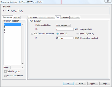
Fig.3. Second window where we can define amplitudes, and propagation constants, etc.
The question remains about destination boundary. Here again we use PORT BC, with H0z set to 0, but propagation constant is the same as in the case of SOURCE PORT. Defined in this way, DESTINATION PORT will absorb incoming wave without any reflection. However if you have scattering object, that scatters a lot, scattered field will be reflected back into geometry, and other BC are necessary.
After pressing mesh button, we can solve the model. Solution will appear as on Fig.4.
IMPORTANT NOTE: When extracting S-parameters or integrating power flow to get T or R parameters, you should not do it on the external boundaries or internal PML boundaries. You should create internal boundary for assessing the required parameters.
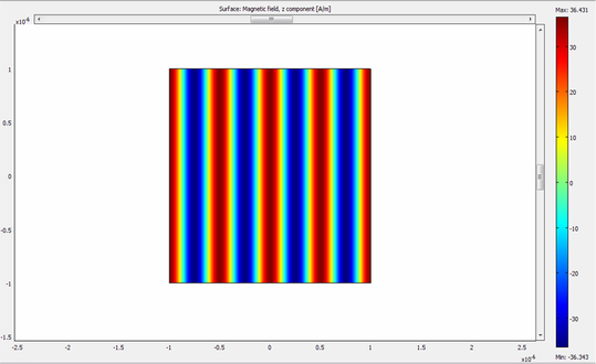
Fig.4. Automatically plotted solution
How to know if meshing is good? First you can visualize Hz and Ey. If you see some grainy picture, you should refine it. In 2D I highly recommend quad meshing, it gives great results. TRY it OUT! Most of times solution looks smooth, and you are not sure if it is ok. I suggest you the simple and very effective test. We know that input power was 0.5W, and since there are no absorbers or scatterers, output power should be the same.Thus, integrate time averaged power on DESTINATION BOUNDARY, and if it is too different from incident, then refine your mesh. It will always be slightly different due to numerrical errors during calculations of the excitation. This is big difference with scattering harmonic propagation formalism. If you set the same model in scattering harmonic propagation, your power at input will be the same as at DESTINATION boundary. Of course this is true, because if there is only empty space, COMSOL will not calculate anything, it will just plot your definition (See other pages)
Instead of closing DESTINATION boundary with absorbing BC, we can introduce PML. If PML is working fine, DESTINATION BC can be almost whatever, because PML will absorb all, before wave even reaches the DESTINATION boundary. Actually, after PML there is no reason to put absorbing PORT BC because we don´t know propagation constant after it travels through PML. The best suited is SC BC, but here you can set PEC or PMC, or whatever, it will not change solution in your geometry. You can test that by integrating POWER on interior PML boundary.
Instead of closing DESTINATION boundary with absorbing BC, we can introduce PML. If PML is working fine, DESTINATION BC can be almost whatever, because PML will absorb all, before wave even reaches the DESTINATION boundary. Actually, after PML there is no reason to put absorbing PORT BC because we don´t know propagation constant after it travels through PML. The best suited is SC BC, but here you can set PEC or PMC, or whatever, it will not change solution in your geometry. You can test that by integrating POWER on interior PML boundary.
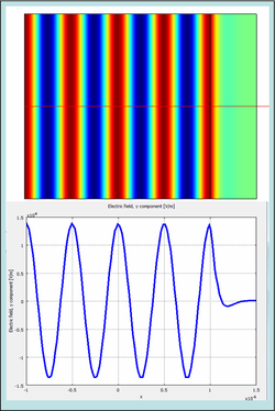
Fig.5. Solution of the same model with PML before DESTINATION boundary. Lower: Plot of Ey through the geometry. Note strong damping in PML area.
In conclusion, you have seen how to set PORT BC in 2D. This is the most simple model possible. The most important thing here is that when defining PORT BC whatever amplitude different than zero is set, it will be disregarded, and will be calculated automatically by COMSOL from input POWER that you set.Propagation constant (Beta) is by definition k-vector component that is normal to the boundary. Later, I will explain how to define oblique excitation, with k-vector that is not parallel to the normal of the SOURCE boundary.
