Proper use of PMLs and BCs with assemblies (2D)
I showed in previous page that PORT or SC BC are absorbing reflected waves with same propagation constant as excited wave. That is consequence of absorbing boundary condition for scattered field in total field formalism. But when there is a scatterer, scattered waves don't have same propagation constant as excited wave. Thus, BC cannot absorb scattered waves. Solution to that situation is implementation of PML that will absorb reflected wave.Generally, you might pass incident wave first through PML before entering geometry, but is not recommended.
ASSEMBLY and IDENTITY PAIRS
By default in COMSOL, when generating geometry, analyzed geometry is represented as single composite object which is consisted of subdmains. If we check Use Assembly option under Draw menu, then we can define parts of geometry to be individual objects. This objects are not connected at all, even if it might look that they have common boundary, if not specified, boundaries are independet, independent BC can be set, and meshing is different.
If we decide to connect these two objects, we can create IDENTITY PAIRS that link physics of both of them. Generally speaking, linked boundaries are not necessary geometrically identical, but in our case they will be always. BC condition can be set for Identity pair which forces dependent variable that can be discontinuous to "obey" to BC of identity pair. If it is continuity BC, it will force dependent variable on destination boundary to be the same as on source boundary. (Usually smaller boundary is destination, and larger is source, but since here we use same boundaries it is not always clear). However we can always exchange source-destination sides in Physics/Identity pairs. When creating Identity pairs you choose objects that are going to be linked, and it is recommended to use Imprint option. Imprint will make that edges of two sides of boundaries coincide when meshing. Meshes can be different, but my experience in RF says that you should use COPY MESH option.
I will use Assembly and Identity pair to insert excitation on otherwise interior boundary, that will allow me to close geometry with PMLs on both sides, as we will see in the following example.
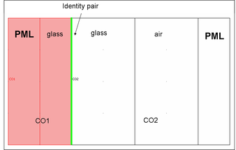
Figure 1. Building up geometry made in Assembly mode
Go to Draw menu and check USE ASSEMBLY. Make your subdomains as in Figure 1. and define material properties and PMLs accordingly. Now select 2 subdomains highlighted in red, and press Draw/Coerce to Solid. That will make single composite object marked CO1. Do the same for three right subdomains, and you will get CO2. Now we have two separate objects, and we have to link them. Go to Draw and click Create pairs... Highlight CO1 and CO2, and press OK. Now if you go to Physics/Boundary settings there is PAIRS tab, where you can set boundary condition that you like. Here we will use PORT BC and set it identically as in previous webpage. Do the meshing, but first mesh one boundary of Identity pair, and use COPY mesh option to generate identical mesh. The rest you can mesh as before. Now you are ready to Solve the model. Solution is shown in Figure 2.
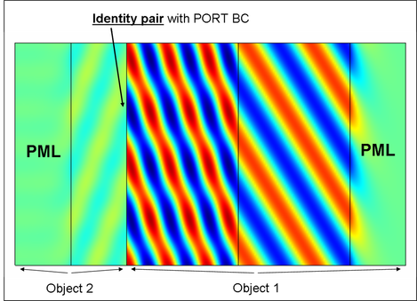
Figure 2. Proper use of PMLs in combination with PORT BC or SC BC in total field formalism. Excitation is set inside modleing domain by the means of Identity Pairs
You can notice that in CO1 there is only reflected wave from glass/air interface. PORT BC ensures that there is a continuity of absorbed wave (reflected wave) that comes toward the boundary with wave on the destination boundary (CO1). Excited wave travels toward interface. If you get situation where incident wave is traveling backwards, although you set your propagation constant in +x direction, just exchange source/destination boundaries in Identity pair, since COMSOL uses this as priority and disregards minus sign in propagation constant.
You can see that solution is same as in the previous page. That is so, because PORT BC can adsorb perfectly reflected wave.But try to put metallic scatterer in both models, and you will notice the difference. You can insert additional boundaries close to inner PML sides, that you will use for calculations of reflectance and transmittance. You can calculate R and T as function of wavelength or angle of incidence, and compare it with some analytical model. Then you can be sure that everything is set well and that chosen mesh is dense enough.
Now you can expand this to 3D case, and you are ready to publish!
